Creative Prediction with Neural Networks
A course in ML/AI for creative expression
Mixture Density Networks
Charles Martin - The Australian National University

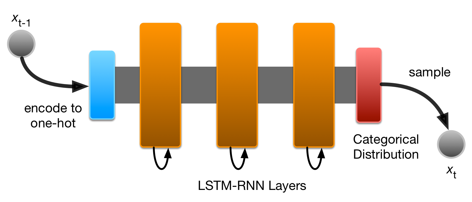
So far; RNNs that Model Categorical Data
- Remember that most RNNs (and most deep learning models) end with a softmax layer.
- This layer outputs a probability distribution for a set of categorical predictions.
- E.g.:
- image labels,
- letters, words,
- musical notes,
- robot commands,
- moves in chess.

Expressive Data is Often Continuous


So are Bio-Signals


Image Credit: Wikimedia
Categorical vs. Continuous Models


Normal (Gaussian) Distribution
- mean (\(\mu\)) and
- standard deviation (\(\sigma\))
The “Standard” probability distribution
Has two parameters:
Probability Density Function:
\[\mathcal{N}(x \mid \mu, \sigma^2) = \frac{1}{\sqrt{2\pi\sigma^2} } e^{ -\frac{(x-\mu)^2}{2\sigma^2} }\]
Problem: Normal distribution might not fit data
What if the data is complicated?
It’s easy to “fit” a normal model to any data.
Just calculate \(\mu\) and \(\sigma\)
(might not fit the data well)

Mixture of Normals
Three groups of parameters:
- means (\(\boldsymbol\mu\)): location of each component
- standard deviations (\(\boldsymbol\sigma\)): width of each component
- Weight (\(\boldsymbol\pi\)): height of each curve
Probability Density Function:
\[p(x) = \sum_{i=1}^K \pi_i\mathcal{N}(x \mid \mu, \sigma^2)\]
This solves our problem:
Returning to our modelling problem, let’s plot the PDF of a evenly-weighted mixture of the two sample normal models.
We set:
- \(K = 2\)
- \(\boldsymbol\pi = [0.5, 0.5]\)
- \(\boldsymbol\mu = [-5, 5]\)
- \(\boldsymbol\sigma = [2, 3]\)
(bold used to indicate the vector of parameters for each component)

In this case, I knew the right parameters, but normally you would have to estimate, or learn, these somehow…
Mixture Density Networks

- Neural networks used to model complicated real-valued data.
- i.e., data that might not be very “normal”
- Usual approach: use a neuron with linear activation to make predictions.
- Training function could be MSE (mean squared error).
- Problem! This is equivalent to fitting to a single normal model!
- (See Bishop, C (1994) for proof and more details)
Mixture Density Networks

- Idea: output parameters of a mixture model instead!
- Rather than MSE for training, use the PDF of the mixture model.
- Now network can model complicated distributions! 😌
Simple Example in Keras

Difficult data is not hard to find! Think about modelling an inverse sine (arcsine) function.
- input value takes multiple outputs…
- is not going to go well for a single normal model.
Feedforward MSE Network
Simple two-hidden-layer network (286 parameters):
model = Sequential()
model.add(Dense(15, batch_input_shape=(None, 1), activation='tanh'))
model.add(Dense(15, activation='tanh'))
model.add(Dense(1, activation='linear'))
model.compile(loss='mse', optimizer='rmsprop')
model.fit(x=x_data, y=y_data, batch_size=128, epochs=200, validation_split=0.15)
Feedforward MSE Network (Result)
Simple two-hidden-layer network (286 parameters):


MDN Architecture:
Loss function for MDN is negative log of likelihood function \(\mathcal{L}\).
\(\mathcal{L}\) measures likelihood of \(t\) being drawn from a mixture parametrised by \(\mu\), \(\sigma\), and \(\pi\) which are generated by the network inputs \(x\): \[\mathcal{L} = \sum_{i=1}^K\pi_i(\mathbf{x})\mathcal{N}\bigl(\mu_i(\mathbf{x}), \sigma_i^2(\mathbf{x}); \mathbf{t} \bigr)\]Feedforward MDN Results
Two-hidden-layer MDN (510 parameters)---works much better!


Some more details….

- This “version” of a mixture model works for a mixture of 1D normal distributions.
- Not too hard to extend to multivariate normal distributions, which are useful for lots of problems.
- This is how it actually works in my Keras MDN layer, have a look at the code for more details…
MDN-RNNs
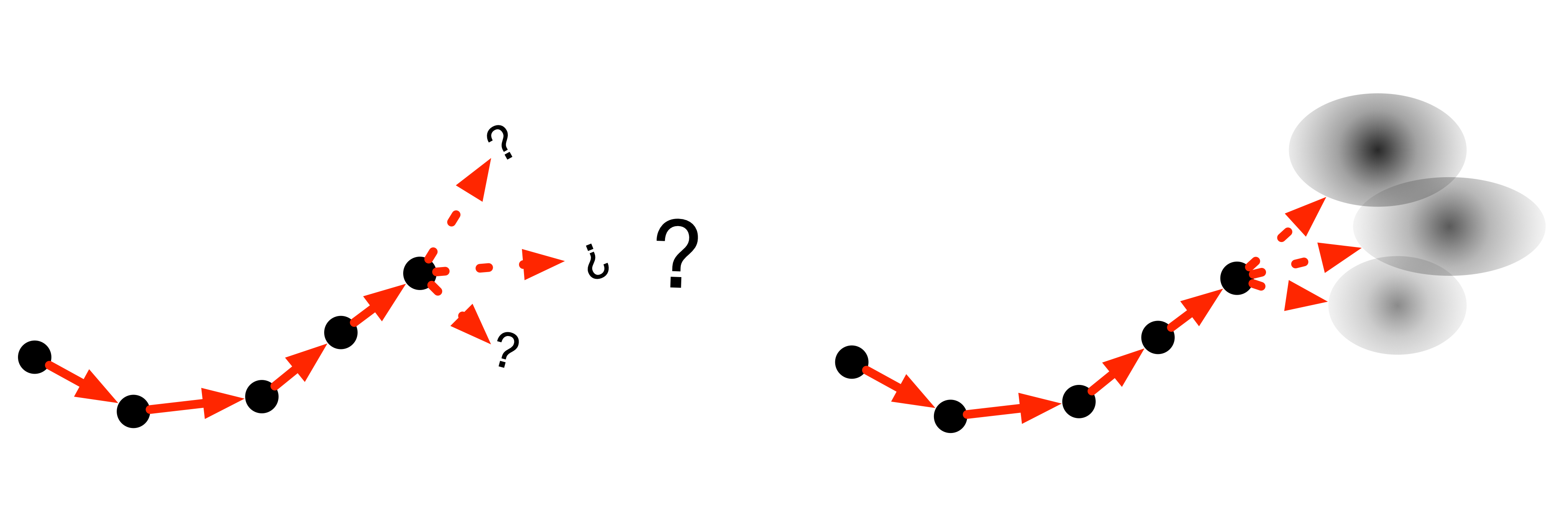
MDNs can be handy at the end of an RNN! Imagine a robot calculating moves forward through space, it might have to choose from a number of valid positions, each of which could be modelled by a 2D Normal model.
MDN-RNN Architecture
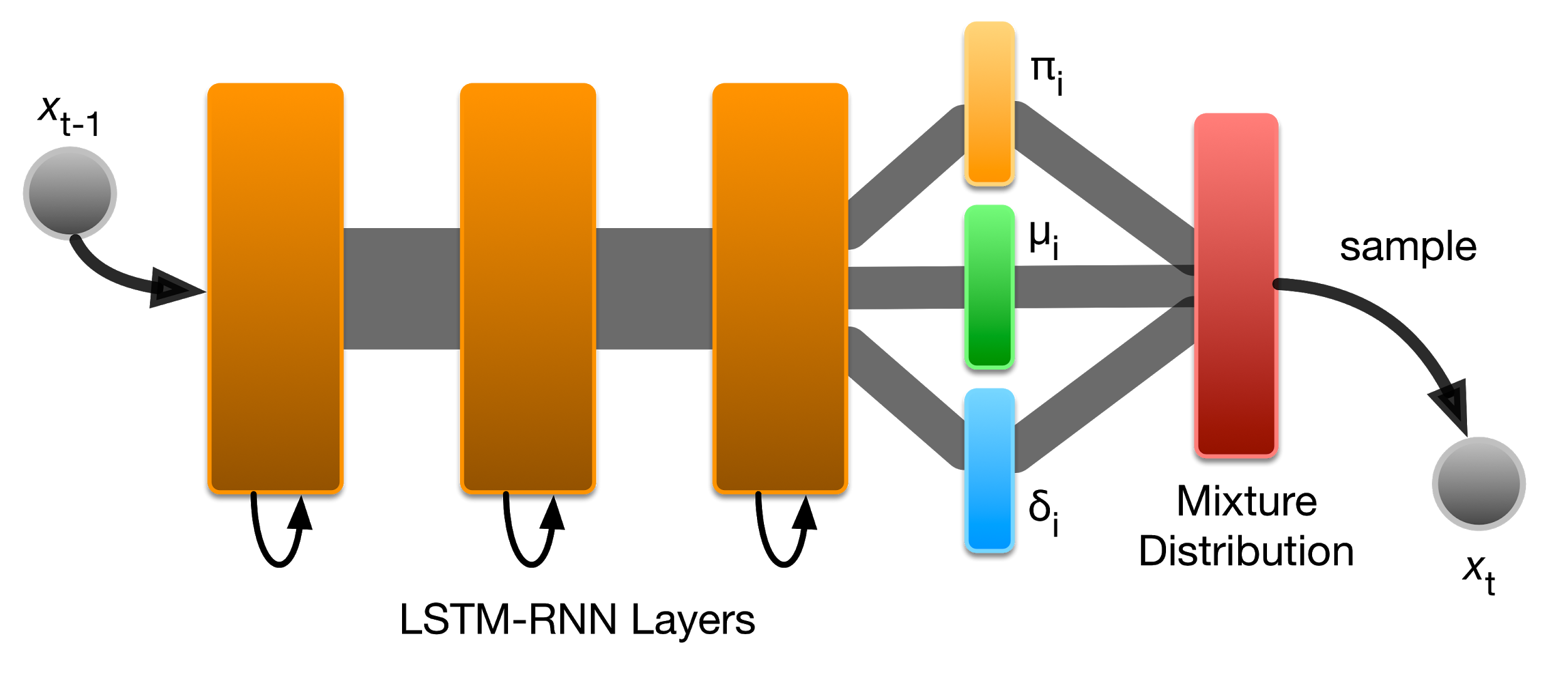
Can be as simple as putting an MDN layer after recurrent layers!
Use Cases: Handwriting Generation


- Handwriting Generation RNN (Graves, 2013).
- Trained on handwriting data.
- Predicts the next location of the pen (\(dx\), \(dy\), and up/down)
- Network takes text to write as an extra input, RNN learns to decide what character to write next.
Use Cases: SketchRNN


- SketchRNN Kanji (Ha, 2015); similar to handwriting generation, trained on kanji and then generates new “fake” characters
- SketchRNN VAE (Ha et al., 2017); similar again, but trained on human-sourced sketches. VAE architecture with bidirectional RNN encoder and MDN in the decoder part.
Use Cases: World Models
- World Models (Ha & Schmidhuber, 2018)
- Train a VAE for visual perception an environment (e.g., VizDoom), now each frame from the environment can be represented by a vector \(z\)
- Train MDN to predict next \(z\), use this to help train an agent to operate in the environment.

